
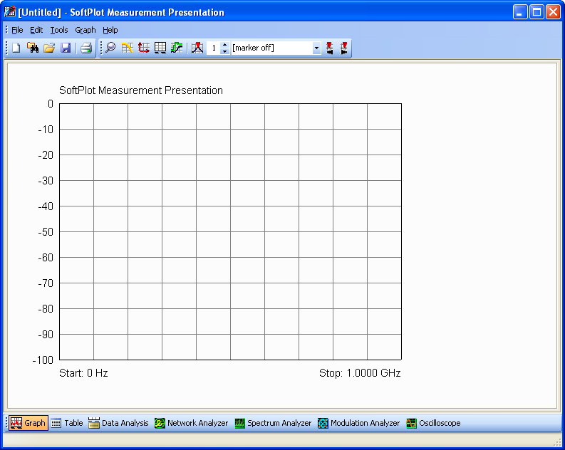
SoftPlot is organised into a number of tabbed pages. The first one shows the Graph, which initially has no traces on it. There are other pages to show the underlying numerical trace data (Table page), the Data Analysis (such as modulation accuracy), and further pages to transfer measurements from your Network Analyzer, Spectrum Analyzer, Modulation Analyzer and Oscilloscope. To extract the trace information from an instrument, switch to the appropriate tabbed page.
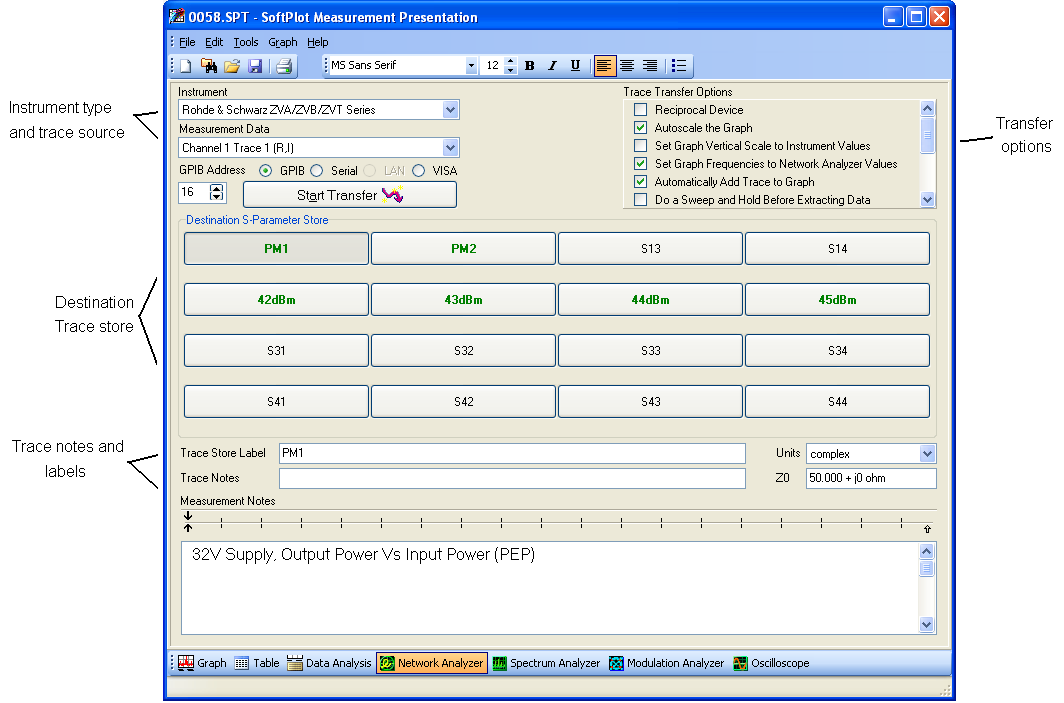
Connect the GPIB cable between instrument and PC, and then select the
instrument type from the list. Check that the address of the instrument is the
same on the SoftPlot screen (note that SoftPlot remembers instrument and address
preferences between sessions). Choose the destination trace store for the
transferred data. Then click on
 , and in a
few seconds, the data has arrived.
, and in a
few seconds, the data has arrived.
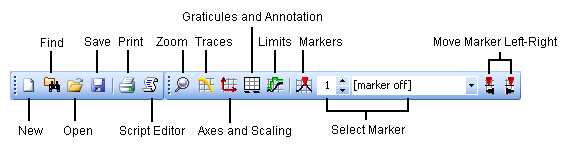
On the graph page is a toolbar for controlling the appearance of the graph. Use the Traces button to choose which trace stores are displayed, and to set trace-specific colours, offsets, etc.
Axes and Scaling is used to set the vertical and horizontal display scales, and to choose the display formatting for each of the vertical axes (log magnitude, phase, real/imaginary part, VSWR, etc). Alternatively, you can zoom in and out interactively with the mouse when the magnifying glass is selected.
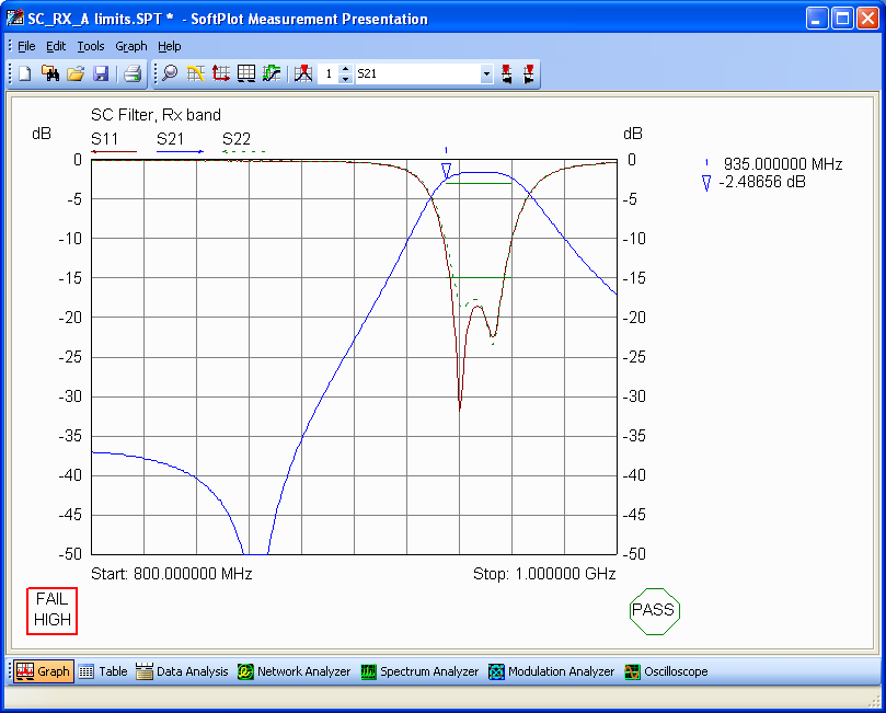
Graticules and Annotation allows the graticule to be optimised to suit the measurement data. There are four styles which emulate each of the supported instrument categories, in addition to a generic style. For example. the oscilloscope style has 8 x 10 squares where the others have 10 x 10 rectangles. The annotation below the graph varies according to the graticule style, so that resolution and video bandwidth are displayed on spectrum analyzer measurements, and symbol period is shown on modulation measurements.
There are over 10 graticule types to choose from. Network analyzer measurements can be redisplayed on a Smith chart (impedance or admittance), or any of the cartesian types, including log-frequency distribution. Modulation measurements can be displayed in constellation form or as an eye diagram, all from the same initial measurement data.
Markers can be set up using the Markers toolbar button, and then moved interactively using the marker controls.
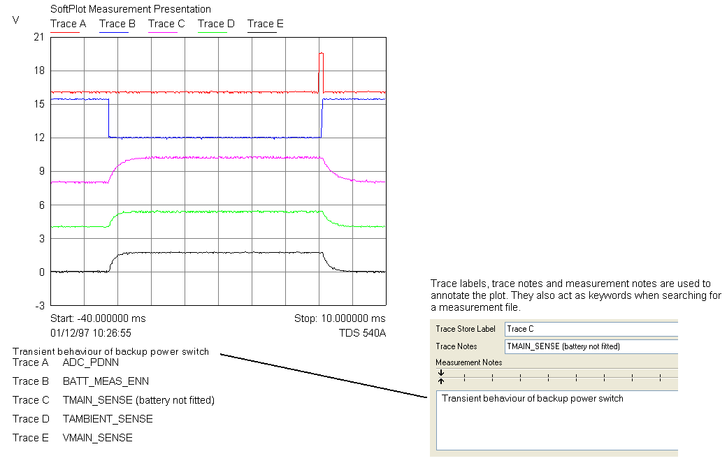
Document your measurements and specific details about each trace using Trace Notes. These can be hidden, or formatted automatically below the graph.
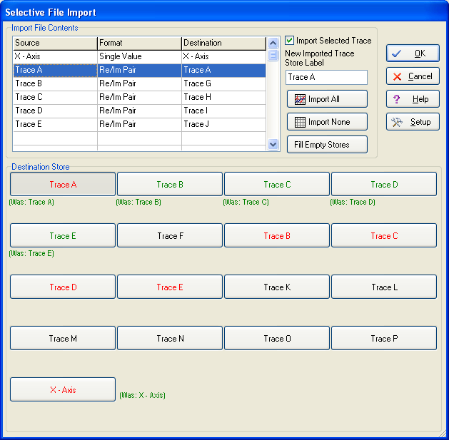
Exporting and importing from other files and file formats is a standard feature in SoftPlot. Particularly important is the ability to merge measurements and style components from other files to assemble a composite graph. Use the Selective File Import function to choose particular trace stores from another file, and to determine which stores in the current file they should fill.
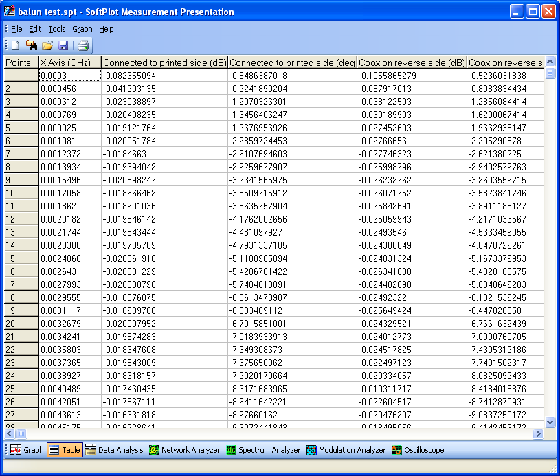
The trace data is available on the Table page as tabular data, much like a spreadsheet. Ranges of cells can be cut and pasted into and from spreadsheet and word processor packages, and individual data points can be entered or edited.
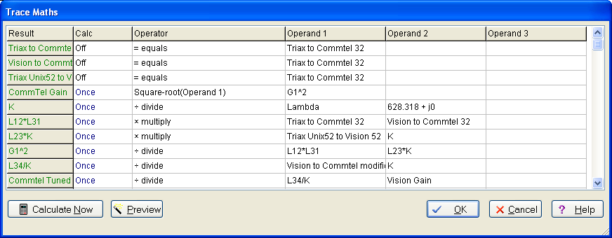
Advanced trace data processing can be carried out with the Trace Maths functions, where new traces can be generated as a result of a range of maths operations.
SoftPlot and Network Analyzers
SoftPlot and Spectrum Analyzers
SoftPlot and Modulation Analyzers
Features Summary, Hardware Requirements, Pricing and Ordering